17 Miscellaneous
This chapter collects a set of “tools of the trade” that show up repeatedly in statistical practice:
linear algebra, calculus, and a few practical workflows (sample size simulation, z-score evaluation, and reproducible reporting with bookdown/blogdown).
The intention is not to present a rigorous proof-based treatment, but to provide a working reference with short explanations and runnable code.
17.1 Linear algebra
Linear algebra is the language of most modern statistical modeling. Regression, mixed models, PCA, and many optimization algorithms are built on matrix representations:
- data are organized as matrices (design matrices),
- parameters are vectors,
- sums of squares become quadratic forms,
- estimation becomes solving linear systems or matrix decompositions.
17.1.1 Matrix basics
17.1.1.1 Dimensions of a matrix
A matrix has two dimensions: number of rows and number of columns. In R, dim() returns both.
| 1 | 5 | 9 |
| 2 | 6 | 10 |
| 3 | 7 | 11 |
| 4 | 8 | 12 |
[1] 4 3[1] 4[1] 3Key ideas:
- dim(X) returns (nrow, ncol).
- dim(X)[1] extracts the number of rows.
- ncol(X) is a convenience function for columns.
17.1.1.2 Change dimensions of a matrix
In R, you can reshape a matrix by changing its dim. This does not change the values, only how they are arranged (by column, because R stores matrices column-wise).
| 1 | 3 | 5 | 7 | 9 | 11 |
| 2 | 4 | 6 | 8 | 10 | 12 |
This is essentially a “reshape” of the underlying vector 1:12.
17.1.1.3 Change names of a matrix
Row and column names improve readability and reduce mistakes, especially when matrices represent parameters or covariance structures.
  a <- matrix(1:6,nrow=2,ncol=3,byrow=FALSE)
  b <- matrix(1:6,nrow=3,ncol=2,byrow=T)
  c <- matrix(1:6,nrow=3,ncol=2,byrow=T,dimnames=list(c("A","B","C"),c("boy","girl")))
c| boy | girl | |
|---|---|---|
| A | 1 | 2 |
| B | 3 | 4 |
| C | 5 | 6 |
Now we can extract and modify the names:
[1] "A" "B" "C"[1] "boy" "girl"| boy | girl | |
|---|---|---|
| E | 1 | 2 |
| F | 3 | 4 |
| G | 5 | 6 |
17.1.1.4 Replace elements of a matrix
Indexing uses [row, col]. Once you can index, you can update values.
[1] 10| 1 | 5 | 9 |
| 2 | 6 | 1000 |
| 3 | 7 | 11 |
| 4 | 8 | 12 |
17.1.1.5 Extract diagonal elements and replace them
The diagonal is often special: identity matrices, variances, and many decompositions depend on it.
[1] 1 6 11| 0 | 5 | 9 |
| 2 | 0 | 1000 |
| 3 | 7 | 1 |
| 4 | 8 | 12 |
17.1.1.6 Create diagonal and identity matrices
diag(c(...))creates a diagonal matrix with those values.diag(k)creates ak × kidentity matrix.
| 1 | 0 | 0 |
| 0 | 2 | 0 |
| 0 | 0 | 3 |
| 1 | 0 | 0 |
| 0 | 1 | 0 |
| 0 | 0 | 1 |
17.1.2 Operations
17.1.2.1 Transpose
The transpose swaps rows and columns. Many matrix formulas (e.g., normal equations) require transpose.
| 0 | 0 | 0 | 0 |
| 5 | 0 | 0 | 0 |
| 9 | 1000 | 1 | 0 |
17.1.2.2 Row/column summaries
Row sums and means are common in data transformations and checking intermediate quantities.
| 1 | 4 | 7 | 10 |
| 2 | 5 | 8 | 11 |
| 3 | 6 | 9 | 12 |
[1] 22 26 30[1] 5.5 6.5 7.517.1.2.3 Determinant
The determinant summarizes properties of a square matrix:
- If det(A)=0, the matrix is singular (not invertible).
- Determinants also appear in multivariate normal likelihoods via |Σ|.
[1] 0.716529317.1.2.4 Addition
Matrix addition requires the same dimensions.
  A=matrix(1:12,nrow=3,ncol=4)
  B=matrix(1:12,nrow=3,ncol=4)
A+B #same dimensions (non-conformable arrays)| 2 | 8 | 14 | 20 |
| 4 | 10 | 16 | 22 |
| 6 | 12 | 18 | 24 |
17.1.2.6 Multiply by a scalar
Scalar multiplication rescales all entries.
| 2 | 8 | 14 | 20 |
| 4 | 10 | 16 | 22 |
| 6 | 12 | 18 | 24 |
17.1.2.7 Matrix multiplication (dot product)
Matrix multiplication requires conformable dimensions:
- if A is m×k, B must be k×n.
Warning in matrix(1:12, nrow = 2, ncol = 4): data length differs from size of
matrix: [12 != 2 x 4]| 50 | 114 | 178 |
| 60 | 140 | 220 |
17.1.2.8 Kronecker product
The Kronecker product appears in block matrix constructions and covariance modeling (e.g., separable covariance).
| 1 | 1 | 3 | 3 |
| 1 | 1 | 3 | 3 |
| 2 | 2 | 4 | 4 |
| 2 | 2 | 4 | 4 |
17.1.2.9 Inverse matrix
A matrix must be square and non-singular to have an inverse. Inverse matrices appear in closed-form least squares and covariance transformations.
| -1.3843051 | -1.310550 | 0.740038 |
| 0.0789580 | 1.051403 | -0.711770 |
| -0.5636427 | 0.738301 | 2.260475 |
| -0.7582116 | -0.9167069 | -0.0404247 |
| -0.0581822 | 0.7085465 | 0.2421523 |
| -0.1700547 | -0.4599988 | 0.3532150 |
| 1 | 0 | 0 |
| 0 | 1 | 0 |
| 0 | 0 | 1 |
The matlib package provides a more explicit inv().
| -0.7582116 | -0.9167069 | -0.0404247 |
| -0.0581822 | 0.7085465 | 0.2421523 |
| -0.1700547 | -0.4599988 | 0.3532150 |
17.1.2.10 Generalized inverse
When a matrix is not square (or is singular), we can use a generalized inverse (Moore–Penrose pseudoinverse). This is common in least squares with rank deficiency.
| 1 | 0 | 0 |
| 0 | 1 | 0 |
| 0 | 0 | 1 |
| -1.3843051 | -1.310550 | 0.740038 |
| 0.0789580 | 1.051403 | -0.711770 |
| -0.5636427 | 0.738301 | 2.260475 |
The product A %*% ginv(A) %*% A is a projection-like operation: it maps back into the column space of A.
17.1.2.11 crossprod
crossprod(B) computes t(B) %*% B efficiently and with better numerical stability.
| 1 | 5 | 9 |
| 2 | 6 | 10 |
| 3 | 7 | 11 |
| 4 | 8 | 12 |
| 30 | 70 | 110 |
| 70 | 174 | 278 |
| 110 | 278 | 446 |
| 30 | 70 | 110 |
| 70 | 174 | 278 |
| 110 | 278 | 446 |
Generalized inverse utilities with crossprod:
| -0.375 | -0.1458333 | 0.0833333 | 0.3125 |
| -0.100 | -0.0333333 | 0.0333333 | 0.1000 |
| 0.175 | 0.0791667 | -0.0166667 | -0.1125 |
| 0.2664931 | 0.0763889 | -0.1137153 |
| 0.0763889 | 0.0222222 | -0.0319444 |
| -0.1137153 | -0.0319444 | 0.0498264 |
17.1.3 Eigen decomposition
Eigen decomposition is defined for square matrices. It is central in: - PCA and spectral methods, - diagonalizing symmetric matrices, - understanding quadratic forms and covariance matrices.
For an m×m matrix A, eigen decomposition takes the form:
- values: eigenvalues (Λ)
- vectors: eigenvectors (U)
In many texts: A = U Λ U^{-1}.
For symmetric matrices, U is orthogonal and U^{-1} = U', giving A = U Λ U'.
17.1.3.1 Eigen values
[1] 1.611684e+01 -1.116844e+00 -5.700691e-16| 16.11684 | 0.000000 | 0 |
| 0.00000 | -1.116844 | 0 |
| 0.00000 | 0.000000 | 0 |
17.1.3.2 Eigen vectors
| -0.4645473 | -0.8829060 | 0.4082483 |
| -0.5707955 | -0.2395204 | -0.8164966 |
| -0.6770438 | 0.4038651 | 0.4082483 |
We can reconstruct A (approximately) using eigenvectors and eigenvalues:
| 3 | 4 | 5 |
| 4 | 5 | 6 |
| 5 | 6 | 7 |
| 1 | 4 | 7 |
| 2 | 5 | 8 |
| 3 | 6 | 9 |
Small discrepancies may occur due to rounding and floating-point arithmetic.
17.1.4 Advanced operations
17.1.4.1 Cholesky factorization
Cholesky factorization applies to symmetric positive definite matrices:
- A = R'R (or sometimes A = LL' depending on convention),
- chol(A) returns an upper triangular factor by default.
Covariance matrices are typically positive semidefinite; in practice, estimated covariance matrices are often treated as positive definite (or adjusted to be so).
| 2 | 1 | 1 |
| 1 | 2 | 1 |
| 1 | 1 | 2 |
| 1.414214 | 0.7071068 | 0.7071068 |
| 0.000000 | 1.2247449 | 0.4082483 |
| 0.000000 | 0.0000000 | 1.1547005 |
Check the reconstruction:
| 2 | 1 | 1 |
| 1 | 2 | 1 |
| 1 | 1 | 2 |
Compute inverse via Cholesky:
| 0.75 | -0.25 | -0.25 |
| -0.25 | 0.75 | -0.25 |
| -0.25 | -0.25 | 0.75 |
| 0.75 | -0.25 | -0.25 |
| -0.25 | 0.75 | -0.25 |
| -0.25 | -0.25 | 0.75 |
Using Cholesky is often numerically preferable to directly calling solve() for symmetric positive definite matrices.
17.1.4.2 Singular value decomposition (SVD)
SVD works for any m×n matrix and is among the most robust matrix decompositions.
A = U D V'
U: orthogonal (m×morm×r)D: diagonal singular values (r×r)V: orthogonal (n×norn×r)r: rank (number of non-zero singular values)
[1] 4.589453e+01 1.640705e+00 1.366522e-15| 1 | 0 | 0 |
| 0 | 1 | 0 |
| 0 | 0 | 1 |
| 1 | 0 | 0 |
| 0 | 1 | 0 |
| 0 | 0 | 1 |
Reconstruction:
| 1 | 4 | 7 | 10 | 13 | 16 |
| 2 | 5 | 8 | 11 | 14 | 17 |
| 3 | 6 | 9 | 12 | 15 | 18 |
| 1 | 4 | 7 | 10 | 13 | 16 |
| 2 | 5 | 8 | 11 | 14 | 17 |
| 3 | 6 | 9 | 12 | 15 | 18 |
SVD is widely used for: - pseudoinverse, - PCA (via centered data matrix), - numerical stability in least squares.
17.1.4.3 QR decomposition
QR is another general decomposition for m×n matrices:
A = Q R
Q: orthogonal (Q'Q = I)R: upper triangular
QR is essential for numerically stable least squares.
$qr
           [,1]        [,2]          [,3]
[1,] -5.4772256 -12.7801930 -2.008316e+01
[2,]  0.3651484  -3.2659863 -6.531973e+00
[3,]  0.5477226  -0.3781696  1.601186e-15
[4,]  0.7302967  -0.9124744 -5.547002e-01

$rank
[1] 2

$qraux
[1] 1.182574 1.156135 1.832050

$pivot
[1] 1 2 3

attr(,"class")
[1] "qr"
Extract the components:
| -0.1825742 | -0.8164966 | -0.4000874 |
| -0.3651484 | -0.4082483 | 0.2546329 |
| -0.5477226 | 0.0000000 | 0.6909965 |
| -0.7302967 | 0.4082483 | -0.5455419 |
| -5.477226 | -12.780193 | -20.083160 |
| 0.000000 | -3.265986 | -6.531973 |
| 0.000000 | 0.000000 | 0.000000 |
17.1.5 Solve linear equations
Many estimation problems reduce to solving Xβ = b.
| 2 | 0 | 2 |
| 2 | 1 | 2 |
| 2 | 1 | 0 |
[1] 1 2 3[1] 1.0 1.0 -0.5If X is singular, solve() fails. In practice, that is a signal to use:
- qr.solve() (least squares),
- ginv() (pseudoinverse),
- or to investigate collinearity/rank deficiency.
17.1.6 Summary
A useful mental map:
- Eigen decomposition: square matrices; reveals directions of stretching/compression.
- SVD: works for any matrix; most robust; basis of pseudoinverse and PCA.
- QR: stable for regression/least squares.
- Cholesky: fastest for symmetric positive definite matrices (especially covariance matrices).
17.2 Calculus
Calculus enters statistical practice in: - optimization (derivatives/gradients), - likelihood theory, - computing integrals for probabilities and expectations.
17.2.1 Derivation
R’s deriv() can symbolically differentiate simple expressions.
expression({
    .value <- x^3
    .grad <- array(0, c(length(.value), 1L), list(NULL, c("x")))
    .grad[, "x"] <- 3 * x^2
    attr(.value, "gradient") <- .grad
    .value
})[1] "expression"[1] 1 8
attr(,"gradient")
x
[1,] 3
[2,] 12We can also request a function output:
[1] "function"[1] 1.224606e-16 -4.898425e-16
attr(,"gradient")
x
[1,] -1
[2,] 1And include constants:
[1] -1
attr(,"gradient")
             x
[1,] -3.464102
Partial derivatives:
[1] 16
attr(,"gradient")
      x  y
[1,] 16 13
In modeling, this kind of derivative structure is the foundation for gradients and Hessians used by optimizers.
17.2.2 Integration
Many probabilities are integrals of density functions.
0.9500042 with absolute error < 0.000000000011 with absolute error < 0.000094Improper integrals (infinite bounds) are supported:
3.141593 with absolute error < 0.000027Trigonometric integrals:
1 with absolute error < 0.00000000000001117.3 Sample size calculation (simulation-based power)
In complex designs, analytic power formulas may not be available or may be hard to trust. Simulation is often more transparent:
- Specify the data-generating process under the alternative,
- simulate many trials,
- apply the intended analysis method,
- estimate power as the proportion of significant results.
Your code implements exactly this idea: for each candidate sample size t, simulate M trials and record whether prop.test() gives p < 0.05.
#given proportion
px3=0.11
px4=0.07
px5=0.08
px6=0.06
px7=0.05

###################

  Outcome0 = NULL

  for (t in seq(350, 600, by=2)){  # change the possible sample size graudally from 400 to 700.

    n=t
    count=0
    M=500   # times of simulation
    for (i in 1:M){

      # for a given sample size (400), for the first simulation,
      # we use rbinom function simulate the contingencey table as below with above given proportions,
      # and calculate the p value by using Chi square test for the simulation
      x3=rbinom(1,n,px3)
      x4=rbinom(1,n,px4)
      x5=rbinom(1,n,px5)
      x6=rbinom(1,n,px6)
      x7=rbinom(1,n,px7)

      data=matrix(c(x3,n-x3,x4,n-x4,x5,n-x5,x6,n-x6,x7,n-x7 ),ncol=2,byrow=T)

      # if the p value of this simulation is less than 0.05, it means we get the significant result for the given this sample size this time. it means we detected the difference in this simulation experiment when the difference is true.
      pv=prop.test(data)$p.value

      count=as.numeric(pv<0.05)+count  #sum of pv<0.05
    }  #end loop of p value
    power0=count/M

    temp <- data.frame(size=t,power=power0)
    Outcome0 =  rbind(Outcome0, temp)
  }  #end loop of power from different sample size

  # generate a new variable named "power_loess" by loess method because the curve of sample size and power is not enough smooth
  power_loess <- round(predict(loess(Outcome0$power ~ Outcome0$size,data=Outcome0,span=0.6)),3)
  Outcome0 =  data.frame(Outcome0, power_loess)

  # plot a line chart of the power and sample size, and smooth the curve by loess method
  plot (Outcome0$size, Outcome0$power,type = "n", ylab = "Power",xlab="Sample size",
        main = expression(paste("Power analysis for GDM")))
  abline(h=0.9,col='red',lwd=2,lty=2)
  abline(h=0.85, col='red',lwd=2,lty=2)
  abline(h=0.8,col='red',lwd=2,lty=2)
  lines(Outcome0$size,power_loess,col="blue",lwd=2)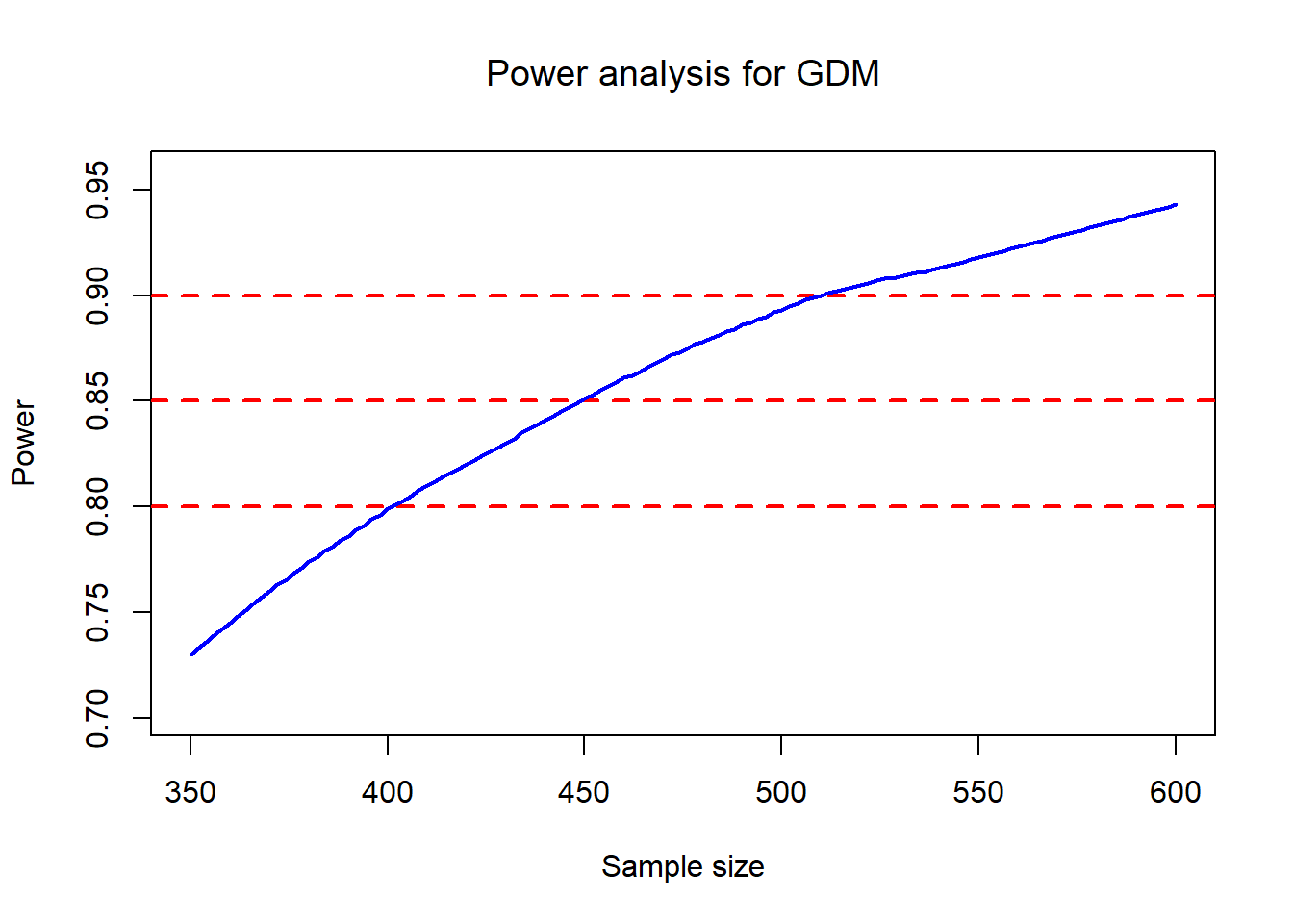
A practical interpretation of the plot:
- The horizontal lines at 0.8 / 0.85 / 0.9 help you read off the required sample size range.
- The loess smoothing stabilizes Monte Carlo noise from finite M.
17.4 How to evaluate a z score
This section demonstrates a common pattern in applied modeling:
- load parameter estimates (here stored in a vector
PE),
- extract the right “row” of estimates for a particular scenario (
Ultra),
- compute mean and variance at a specific time/value
i,
- compute a z-score comparing an observed value to the model-implied distribution.
17.4.1 Call the parameter estimates file
You define which scenario to use:
Then you load a long parameter vector. Conceptually, this is like reading from a saved model object, but stored explicitly as numeric values.
Next, you reshape PE into rows and then select the relevant row using Ultra.
PE= matrix(PE,nrow=5,byrow = T)
    index= Ultra-3;
    info= PE[index,]
    fcoef=info[3:9]; sigma=info[10];Sigmab= matrix(info[11:26],4,4);Zeta=info[27:29];varfixed= matrix(info[30:78],7,7)
    #abstract specific parameters to calculate mean and SD
Interpretation of the objects you create:
- fcoef: fixed-effect coefficients for a spline-like mean function (7 terms).
- sigma: residual SD (or residual scale parameter, depending on model).
- Sigmab: random-effect covariance matrix (4×4), used with Rxxi.
- Zeta: knot locations for truncated power spline terms.
- varfixed: covariance matrix of fixed effects (7×7) used for uncertainty in the mean function.
This decomposition matches how mixed models often separate: - residual variance, - random effect variance, - and uncertainty of estimated fixed effects.
17.4.2 Calculate mean and standard deviation at a specific value
You set i = 28.29 and build two design vectors:
- Fxxi: 7 columns (fixed effects, including spline terms),
- Rxxi: 4 columns (random effects).
i = 28.29
    int <- 1
    t1 <- i
    t2 <- i**2
    t3 <- i**3
    tt1 <- (i - Zeta[1])**3 * (i > Zeta[1])
    tt2 <- (i - Zeta[2])**3 * (i > Zeta[2])
    tt3 <- (i - Zeta[3])**3 * (i > Zeta[3])

    Fxxi = cbind(int, t1, t2, t3, tt1, tt2, tt3)
    Rxxi = cbind(int, t1, t2, t3)

    mean <- Fxxi%*%fcoef
    var <- sigma**2 + Rxxi%*%Sigmab%*%t(Rxxi) + Fxxi%*%varfixed%*%t(Fxxi)
    std <- sqrt(var)
What the variance formula is doing:
- sigma^2: measurement noise / residual variance.
- Rxxi Σ_b Rxxi': variance contributed by random effects at point i.
- Fxxi Var(β) Fxxi': uncertainty from estimating fixed effects (mean curve uncertainty).
17.4.3 Output the calculated mean (on exp scale)
The model seems to operate on the log scale, so exp(mean) returns the mean on the original scale.
Actual Mean= 9.35807117.5 Mathematical coupling
This is a classic example of “leakage”: you create a feature (cuty) derived from the outcome and then include it as a predictor.
Because cuty is essentially a coarsened version of y1to9, it explains a large fraction of the variation and can make the genuine predictors look nonsignificant.
set.seed(1234)   # Random seed
x1 <- rnorm(1000)  #Normal IVs
x2 <- rnorm(1000)
x3 <- rnorm(1000)

yraw <- x1 + x2 + x3 + rnorm(1000,0, 10)
y1to9  <- (yraw + -1*min(yraw)  + 1)
y1to9  <- trunc(y1to9*(9/(max(y1to9))))  #Create a Y variable that goes 1 to 9


cuty <- cut(y1to9,5)
head(cuty)
[1] (1.8,3.6] (3.6,5.4] (3.6,5.4] (5.4,7.2] (5.4,7.2] (1.8,3.6]
Levels: (-0.009,1.8] (1.8,3.6] (3.6,5.4] (5.4,7.2] (7.2,9.01]
Call:
lm(formula = y1to9 ~ x1 + x2 + x3)

Residuals:
    Min      1Q  Median      3Q     Max
-4.0798 -0.8990  0.0888  1.0473  4.8964

Coefficients:
            Estimate Std. Error t value Pr(>|t|)
(Intercept)  3.79492    0.04470  84.899  < 2e-16 ***
x1           0.13592    0.04488   3.029  0.00252 **
x2           0.14269    0.04564   3.126  0.00182 **
x3           0.12522    0.04417   2.835  0.00468 **
---
Signif. codes:  0 '***' 0.001 '**' 0.01 '*' 0.05 '.' 0.1 ' ' 1

Residual standard error: 1.412 on 996 degrees of freedom
Multiple R-squared:  0.02715,   Adjusted R-squared:  0.02422
F-statistic: 9.265 on 3 and 996 DF,  p-value: 0.000004786
model2 <- lm(y1to9~x1 + x2 + x3 + cuty) # Adding the cut of y
summary(model2) #X1, x2, x3 not sig; R^2 is 0.75
Call:
lm(formula = y1to9 ~ x1 + x2 + x3 + cuty)

Residuals:
    Min      1Q  Median      3Q     Max
-0.8743 -0.4458  0.1291  0.4295  0.8184

Coefficients:
               Estimate Std. Error t value Pr(>|t|)
(Intercept)     0.84267    0.06897  12.218   <2e-16 ***
x1              0.02187    0.01540   1.420    0.156
x2              0.01360    0.01567   0.868    0.386
x3              0.01324    0.01516   0.873    0.383
cuty(1.8,3.6]   1.77791    0.07342  24.214   <2e-16 ***
cuty(3.6,5.4]   3.59343    0.07243  49.611   <2e-16 ***
cuty(5.4,7.2]   5.40203    0.08464  63.825   <2e-16 ***
cuty(7.2,9.01]  7.37863    0.25190  29.292   <2e-16 ***
---
Signif. codes:  0 '***' 0.001 '**' 0.01 '*' 0.05 '.' 0.1 ' ' 1

Residual standard error: 0.4821 on 992 degrees of freedom
Multiple R-squared:  0.8871,    Adjusted R-squared:  0.8863
F-statistic:  1113 on 7 and 992 DF,  p-value: < 2.2e-16
The plot illustrates why: cuty is nearly a deterministic summary of the response.
df <- data.frame(cuty, y1to9)
# it causes the coefficient of x1 is 1; others equal 0.
library(ggplot2)
ggplot(data = df,
       mapping = aes(as.numeric(cuty), y1to9)) +
  geom_point() +
  geom_smooth( method = "lm")
`geom_smooth()` using formula = 'y ~ x'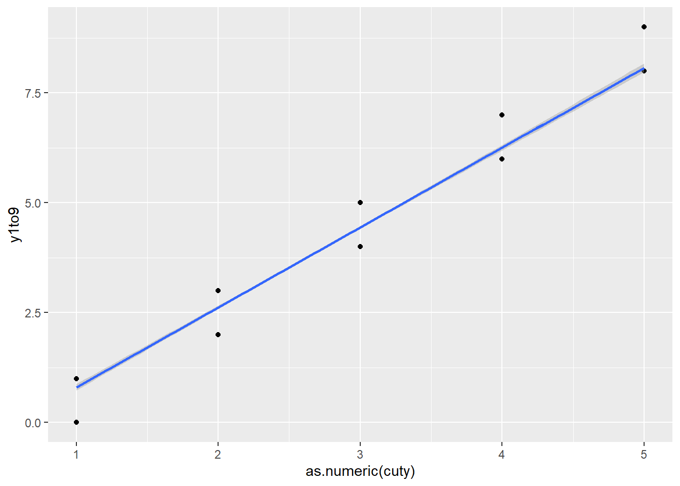
Practical takeaway: - Never include variables derived from the outcome as predictors (unless your modeling framework explicitly accounts for it, such as certain joint models or measurement models). - This problem is common in ML workflows too (target leakage).
17.6 How to create a bookdown
Bookdown is a workflow for writing a multi-chapter book using R Markdown. The main benefits are: - consistent formatting across chapters, - automatic cross-references and numbering, - easy publishing via GitHub + Netlify (or other hosting).
Your steps outline a typical production path:
- create a GitHub repository
- create a new RStudio project using version control
- create and organize
.Rmdchapter files (chapter order determined by filenames) - configure theme and output options (often via
_bookdown.ymland_output.yml) - build locally
- commit and push
- deploy on Netlify, then map to your website
Because bookdown chapters are file-based, naming conventions matter (e.g., 01-intro.Rmd, 02-methods.Rmd, …).
17.6.1 How to git up a project into GitHub
Your notes reflect the standard flow:
- initialize version control in RStudio
- create an empty GitHub repo (no README if you want to push your existing structure cleanly)
- connect local → remote, commit, push
17.6.2 How to git down a project into your PC
Cloning a repo is the reproducible way to move projects across machines: - create project from version control - paste the repo URL - pull and work locally
17.6.3 How to return to a previous version
Downloading and copying works, but in professional workflows you typically:
- use git tags/releases,
- or git checkout <commit> / git revert,
- then commit the rollback.
Your “download then replace” approach is simple and safe for non-technical users, especially if you want to avoid dealing with git history commands.
17.7 How to create a blogdown
Blogdown is more configuration-heavy than bookdown because websites require: - theme configuration, - content organization (posts, pages), - an index page, - and often Hugo theme settings.
You already listed a tutorial and your own blog post as references:
- tutorial: https://www.youtube.com/watch?v=BHpkLJieXPE
- your post: https://danielhe.netlify.app/post/how-to-create-a-blog/
17.8 How to install tensorflow and keras
Your steps reflect the classic RStudio workflow:
- install R packages (tensorflow, keras, reticulate)
- install miniconda
- create/manage a Python environment
- install TensorFlow/Keras into that environment
The key operational points:
- reticulate::install_miniconda() sets up Python.
- install_tensorflow() / install_keras() install Python dependencies.
You included a YouTube tutorial link: https://www.youtube.com/watch?v=cIUg11mAmK4
17.9 How to use GitHub in a team
Your checklist covers the core collaboration pattern:
- clone the repository
- configure username/email
- create a branch per feature or task
- commit and push to that branch
- open a pull request
- merge after review
- pull main regularly
And a set of practical “misc” commands for cleanup and recovery:
- delete branches,
- check status,
- merge,
- manage remotes,
- use reflog/reset/revert cautiously,
- reinitialize or remove .git when needed.
This is the same workflow used by most industry teams.
17.10 How to insert a picture indirectly in markdown
This chunk loads tooling for clipboard-based image insertion.
You included the project link: [link] (https://github.com/Toniiiio/imageclipr)